The data
In this post, I use tick-data of U.S. Dollar Futures contracts traded at BM&F Bovespa. The specifications of this financial asset are given here. I use the data from raw messages available at ftp://ftp.bmf.com.br.
More specifcally, I analyze the U.S. Dollar Futures contracts at March 3rd 2017, with maturity in April, 2017. The code of this asset is DOLJ17.
The goal of this post:
First, we present basic statistics and a visual representation of the U.S. Dollar Futures contract, DOLJ17, for a given day. The basic statistics cover the trades and the limit order book events.
We recall the definition of the Order Book Imbalance and analyze the number (and percentage) of buy and sell market orders that arrive at five different regimes of imbalance. As it was expected from the intuition and other markets, buy (sell) market orders tend to arrive more at regimes of higher (lower) order book imbalance.
Basic Statistics and Visual Representation
We compose the trading data selecting all aggressive market orders executed against orders sited at the limit order book. Moreover, we can see the best limits with dots representing the trades. These dots are proportional to the trade volume. To compare trades with the limit order book, we draw the best limits just prior any given trade.
Next, we see the basic statistics of limit and market orders. In table Trading Statistics, I present the the trades divided into buy and sell market orders. The label Price must be interpreted as the trading prices, being either buy or sell.
Trading Statistics
| index | Price Trade Buy MO | Price Trade Sell MO | Price |
|---|---|---|---|
| count | 20613.00 | 19592.00 | 40205.00 |
| mean | 3178.37 | 3179.04 | 3178.70 |
| std | 10.81 | 10.78 | 10.80 |
| min | 3156.00 | 3079.00 | 3079.00 |
| 25% | 3170.50 | 3171.50 | 3171.00 |
| 50% | 3177.50 | 3178.00 | 3177.50 |
| 75% | 3183.00 | 3183.62 | 3183.50 |
| max | 3300.00 | 3206.00 | 3300.00 |
Limit Order Book Statistics
| index | Bid Price0 | Ask Price0 | Bid Volume0 | Ask Volume0 |
|---|---|---|---|---|
| count | 220912.00 | 220912.00 | 220912.00 | 220912.00 |
| mean | 3178.19 | 3178.80 | 84.37 | 89.74 |
| std | 10.59 | 10.61 | 104.13 | 103.82 |
| min | 3157.50 | 3158.00 | 5.00 | 5.00 |
| 25% | 3171.00 | 3171.50 | 25.00 | 25.00 |
| 50% | 3177.00 | 3178.00 | 55.00 | 60.00 |
| 75% | 3183.00 | 3183.50 | 105.00 | 110.00 |
| max | 3206.00 | 3206.50 | 1290.00 | 1130.00 |
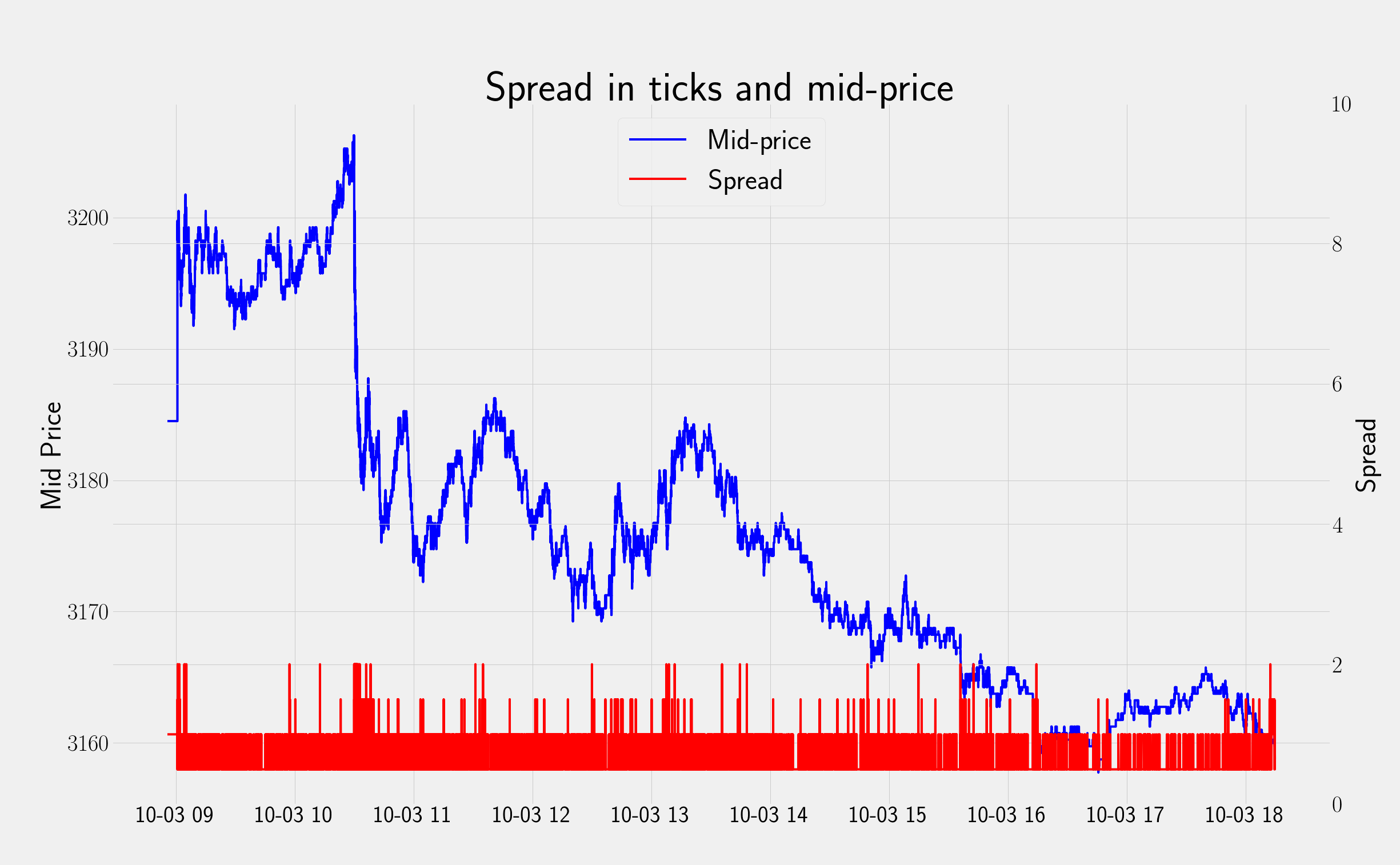
Spread and mid-price
To have a flavor of intraday price variations, in Figure 1 we the mid-price. The mid-price is the average between the best bid and best ask quotes of a given financial asset.
Moreover, in Figure 1 we also illustrate the spread (on the right y axis). The spread is the difference between the best bid and ask quotes. In this example, we show the spread in tick-size. For DOLJ17, the tick-size is R$ 0.5.
Mid-price
Quotes, trades, and volume proportional to trade
Here, we plot six minutes of activity of the first limits together with the trades that happend in this period. The light colored red (blue) dots represent the available quantity at best ask (bid). The dark colors represent the transactions corresponding to each side. The size of the dots are proportional to the size of the transactions.
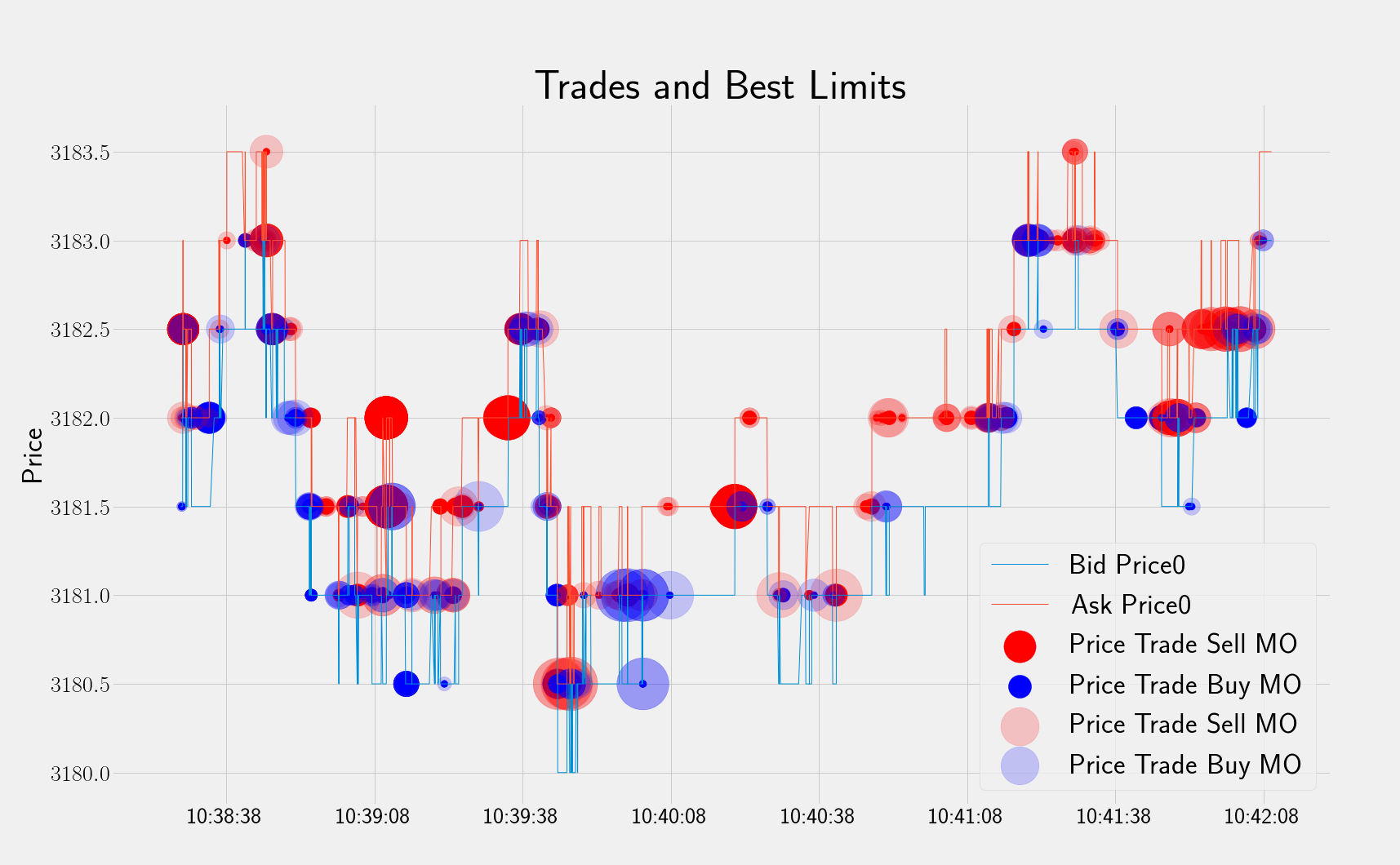
Best bid and ask quotes and trades. The Blue (red) dots represent buy (sell) market orders. The dots size are proportional to the trade volumes.
Order Book Imbalance
The Order Book Imbalance is the difference between the best bid and best ask quantity quotes divided by its sum. That is, $$ Imb_t = \frac{V^{b}_t-V^{a}_t}{V^b_t+V^{a}_t}, $$ where $V_t^{b}$ and $V_t^{a}$ denotes the volume posted at the best bid and at the best ask, respectively.
The Order Book Imbalance measures whether the limit order book is buy or sell heavy. In fact, it is a good predictor of price direction. To illustrate this, in Figure 3 we plot the order imbalance for each quote at the best limits. In this figure, the blue and red dots represent the level of imbalance when buy and sell market orders arrive, respectivelly. Note that Figure 3, the time range is the same as in Figure 2.
Moreover, the inner space between the horizontal lines in Figure 3 represent the imbalance regimes. These regimes are divided in regions such that $Imb_t$ belogs to one of the follwing sets,
$${{[-1, -0.6), [-0.6, -0.2), [-0.2, 0.2), [0.2,0.6), [0.6,1]}}.$$
Note that in Figure 3 we have only three minutes of market activity. If we consider the whole trading day, and count the number of buy and sell market orders conditional on imbalance regimes, we obtain the next Table (see Number of Market Orders). The corresponding bar plot is given in Figure 4. It is interesting to note that in the regimes 4 and 5, the buy market orders dominate the sell market orders. Correspondingly, in the regimes 1 and 2, the sell market orders dominate the buy market orders.
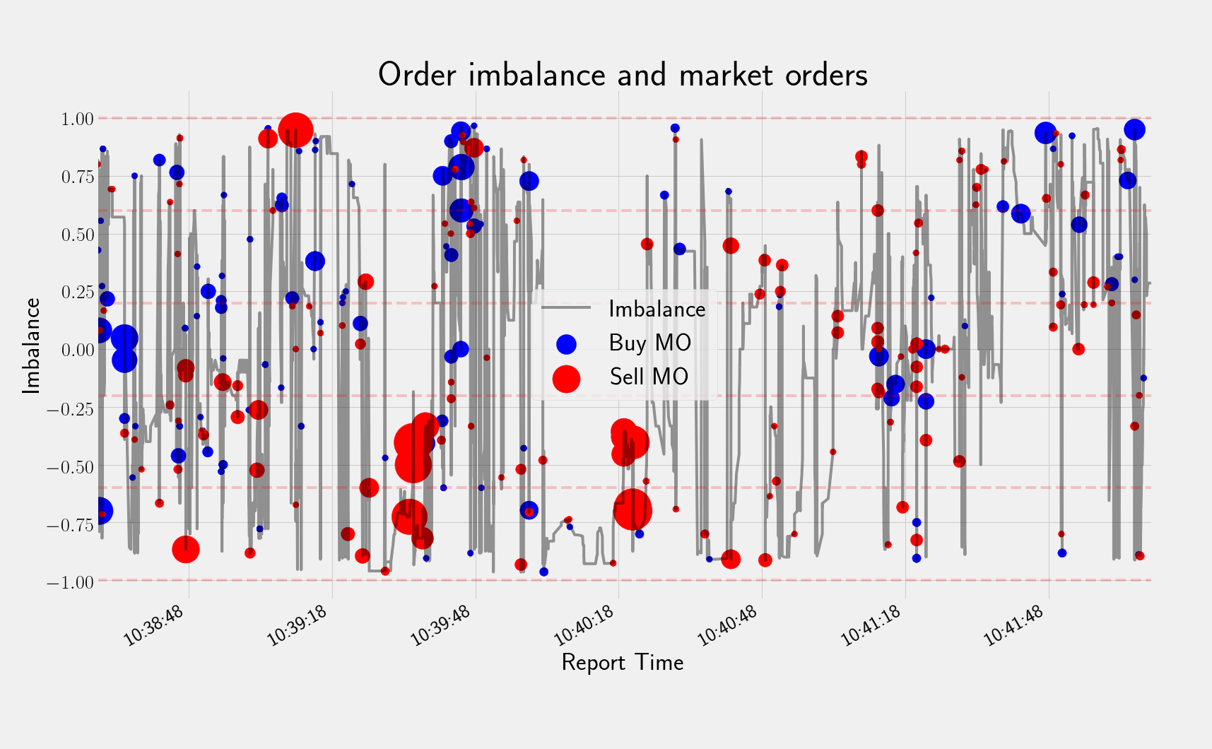
Order imbalance for each quote at the best limits. The blue (red) dots represent Buy (Sell) market orders. The dots size are proportional to the trade volumes.
Number of Market Orders
| Regime | Imbalance Buy MO | Imbalance Sell MO | Total Imbalance |
|---|---|---|---|
| Regime1 | 3858 | 4490 | 8348 |
| Regime2 | 3806 | 4286 | 8092 |
| Regime3 | 4432 | 4456 | 8888 |
| Regime4 | 4411 | 3216 | 7627 |
| Regime5 | 3840 | 2983 | 6823 |
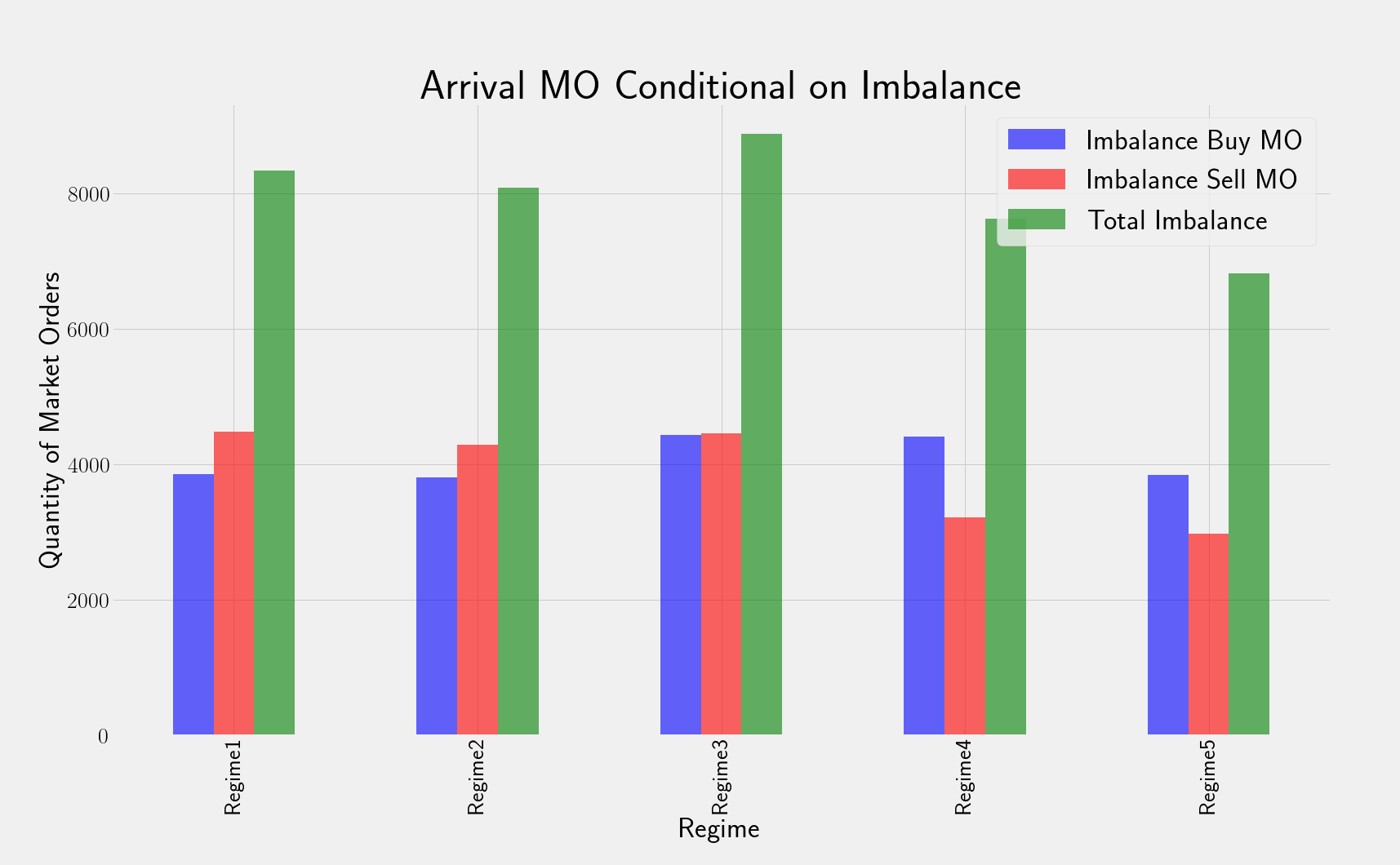
Number of trades conditional on order imbalance regime.
However, the discrepancies between buy and sell market orders are mitigated when we consider the percentage of market orders among the different regimes. Figure 5 must be interpreted as follows. The blue (red) bars represent the proportion of orders, in each regime, of buy (sell) market orders. The sell market orders tend to arrive in regimes with lower imbalance. Hence, we can expect that the market is sell heavy when the imbalance is negative (especially when it is close to -1). Accordingly, the buy market orders tend to occur more in regimes with higher order book imbalance.
Percentage of Makret Orders
| Regime | Imbalance Buy MO | Imbalance Sell MO | Total Imbalance |
|---|---|---|---|
| Regime1 | 18.96 | 23.11 | 20.99 |
| Regime2 | 18.71 | 22.06 | 20.34 |
| Regime3 | 21.78 | 22.93 | 22.34 |
| Regime4 | 21.68 | 16.55 | 19.17 |
| Regime5 | 18.87 | 15.35 | 17.15 |
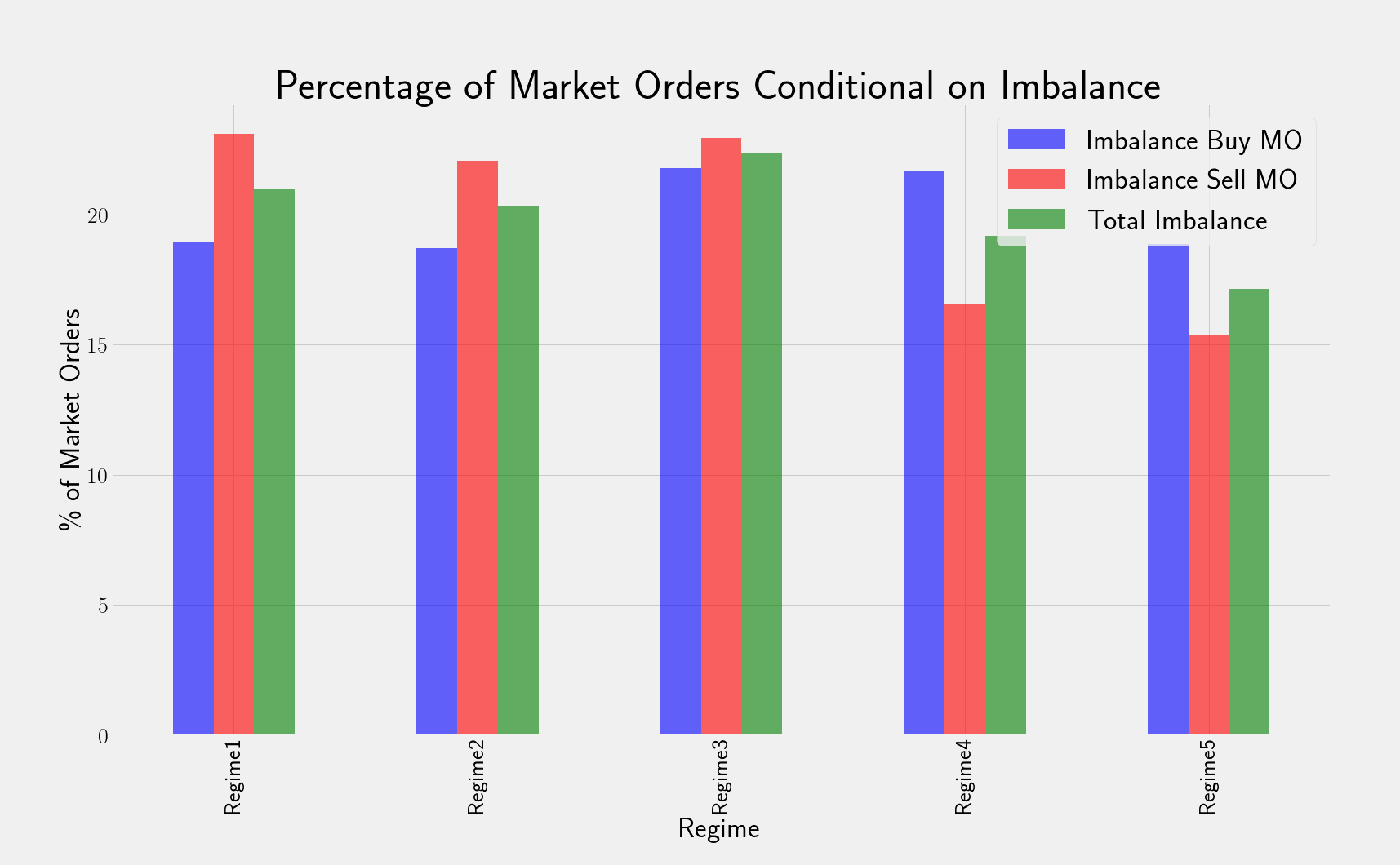
Percentage of trades conditional on order imbalance regime.
Finally, the next Table (see Average Imbalance) shows the average Imbalance just prior the trades arriving at each imbalance regime. The corresponding bar plot is given in Figure 6.
Average Imbalance
| Regime | Imbalance Buy MO | Imbalance Sell MO | Total Imbalance |
|---|---|---|---|
| Regime1 | -0.77936 | -0.792780 | -0.786069 |
| Regime2 | -0.39146 | -0.390470 | -0.390965 |
| Regime3 | 0.01264 | 0.002913 | 0.007777 |
| Regime4 | 0.40137 | 0.402312 | 0.401842 |
| Regime5 | 0.81231 | 0.792619 | 0.802467 |
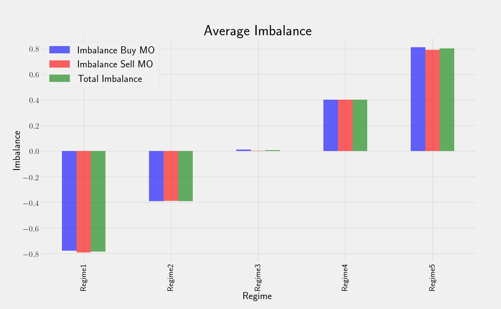
Average of order imbalance when trade occur conditional on order imbalance regime.
Acknowledgement: I would like to thank Rafael Lacerda for providing the data and for the valuable discussions.